
This latest post/spreadsheet demonstrates how to calculate rolling averages and exponentially weighted moving averages, considering for rest days and days with zero data, without the need for entering data with zeros in them for each athlete on these days.
Previously I have shown how to calculate the EWMA in a previous post here, so I won’t go into that in this post. This post will just show the equations used to generate data for every day in a full year for the 20 athletes in this spreadsheet.
I have basic data set which shows date, athlete name, rpe, duration and session load only for the days where there has been training sessions.
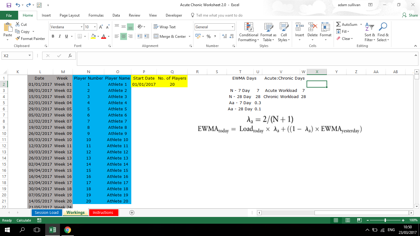
I have set up some columns that have the date and week number, the player number and corresponding name, and then the start date and number of players. The number of players is important because it allows us to display every date for an entire year for each athlete automatically. In the spreadsheet, you will find that every 20 cells the date automatically changes to the next day, which corresponds to the athlete name changing back to repeat the order names.
The first cell in the date column just copies the start date in cell P2, but the next column has the formula =IF(COUNTIF($B$2:B2,B2)<$Q$2,B2,B2+1).
Essentially this equation adds 1 onto the date in cell B2 once the date has been copied down 20 times, since Q2 has 20 in the cell. Adding one onto a date means the next day will be displayed in date format. Cell B22 now shows the next date after the starting date with this formula.
To get player names to repeat you will combine the index, mod and rows formula together.
=INDEX($O$2:$O$21, MOD(ROWS($N$2:N2)-1,$Q$2)+1)
The index function will retrieve data from an array, in this case the array is the player number and the player name. Since we are dealing with numbers and using the number of player’s cell in this formula, then we need to assign each athlete a number.
The rows function tells us the number of rows in the array (player number and player name), in this case there are 20 rows.
The mod function divides the number of rows by the number of players in cell Q2 – every time you get a zero from the mod function alone it means the data will continue in the order of the array you are taking from. For example, when you divide 1,2,3 by the number in Q2 (20) you get zero, but when you hit row 20 you get 1, this is where the data from the array will go back to the first number and repeat the sequence.
But this means when you hit athlete 20 it will change instead of athlete 1 on the next day, in the formula I have put a -1 in, which means the first athlete number (which is 1), will start at zero, the mod function will divide 0 by 20 and get zero so now we get 20 rows from 1 to 20 and not a change on the 20th row.
We add the +1 at the end to allow the index function to get the names up to 20 and then restart all over again.
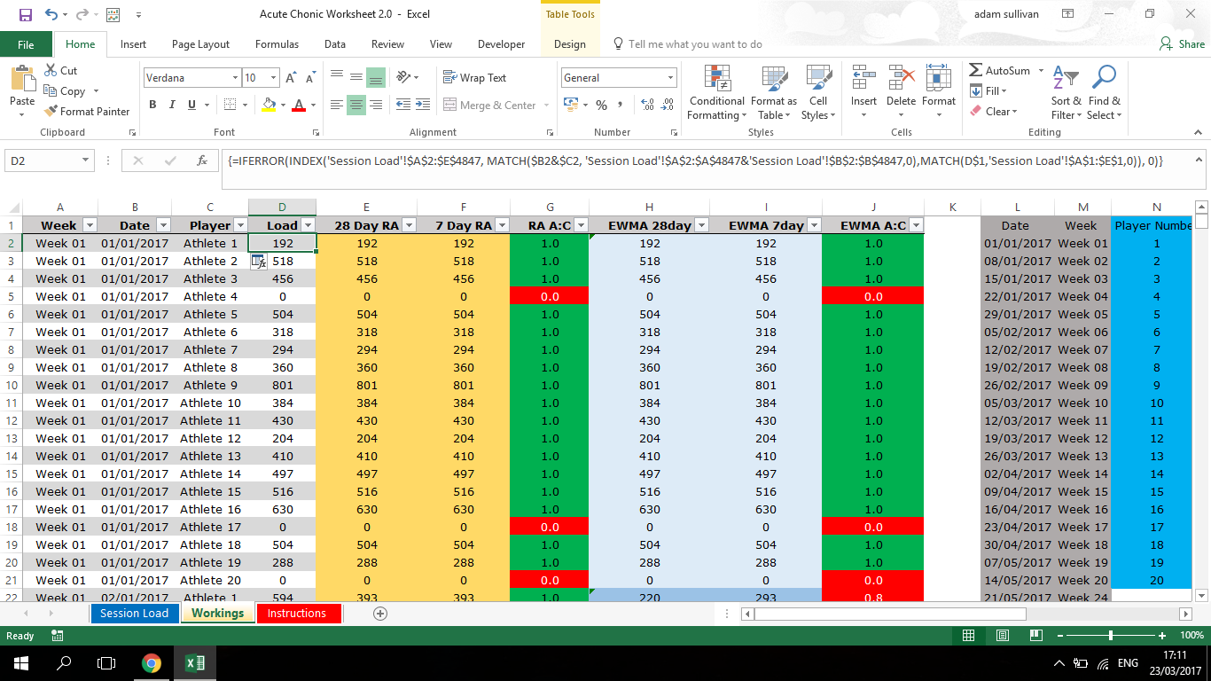
Once you have 20 dates for each date and 20 athletes for each date in order, then you can use these two variables to search the workload for each athlete and corresponding date. Then it’s time to put the index function into the load column, this searches the session load tab from cells A2 to E4847, where all the data collected is, it takes the values in B2 (date) and C2 (athlete) and matches them with the dates in column A and B in the session load tab. Finally, it returns the value matching in the load column – cell D1 in the workings column is the load column, excel needs to look for this heading out of the five headings in the session load tab and return a value from this column that corresponds to the date and athlete.
The IFERROR function before the index formula and the last zero in the formula mean that instead of returning #n/a for an error in the formula, (which occurs when the formula doesn’t return a value) it will return 0.
=IFERROR(INDEX(‘Session Load’!$A$2:$E$4847, MATCH($B2&$C2, ‘Session Load’!$A$2:$A$4847&’Session Load’!$B$2:$B$4847,0),MATCH(D$1,’Session Load’!$A$1:$E$1,0)), 0)
Once you have the date ranges, athlete names and formulas set up to extract the load for a certain date and athlete, then the rolling average calculations are straightforward, and have been demonstrated in the previously mentioned EWMA VS RA post.
Instructions come with the spreadsheet on how to modify it to your needs! Enjoy!
