
Most of the donkey work on this was done by Sean Williams @statman_sean, this project was inspired by the work from David Carey @dlcarey88 and co, in his recent paper on Optimizing Pre-Season Training Loads in Australian Football.
This paper looked at the daily loads and periodisation strategy that would produce the largest total distance covered across pre-season, whilst keeping ACWR and cumulative loads within specified constraints.
Sean put together a mock loading template to replicate this idea by using solver in Excel, the original paper had used MATLAB for its simulations. He was kind enough to send this file to me to try improve, and offer it to be put up here for download!
This tool gives a rough loading template based on specific constraints that you can modify to suit your training/match schedule. Some practical applications of such a method, as mentioned in David Carey’s paper, may be:
- Changing the training loads to gps total distance or another metric of your choice. That might allow coaches to see what may occur when you increase your ACWR max to 1.7, for example. You may end up seeing that you cover an extra 10 km in total distance across the pre-season period at this ratio.
- Planning a safe return to play protocol, perhaps by using more strict ratios and max training loads.
- Developing a training plan that maximises performance/fitness whilst keeping within specific acute to chronic ratios or other variables that can reduce risk of injury.
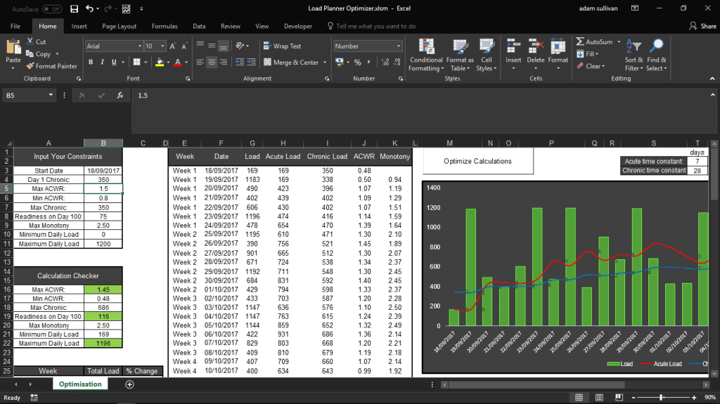
I’ve played around with it by adding a VBA and calculation button in, to allow users to change the constraints by changing the value in certain cells, without diving into solver.
So what is solver?
Solver is part of what-if analysis tools. With Solver, you can find an optimal (maximum or minimum) value for a formula in one cell — called the objective cell — subject to constraints, or limits, on the values of other formula cells on a worksheet. Solver adjusts the values in the decision variable cells to satisfy the limits on constraint cells and produce the result you want for the objective cell. (Microsoft Definition)
Once we go through this process you’ll have a good idea of how solver works!
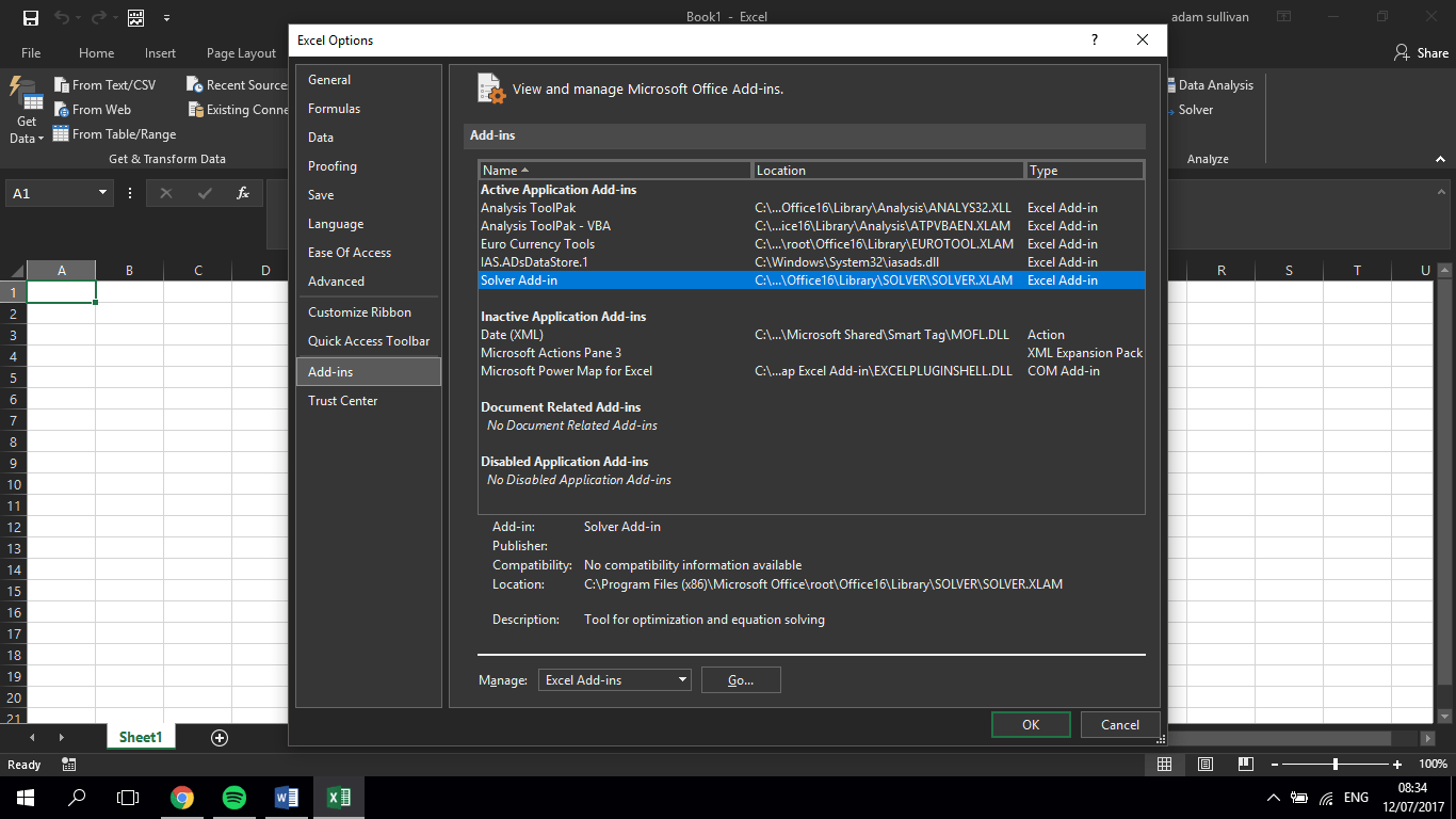
First, check if you have solver installed already, click on the data tab, on the far right should be a section called analyze, here you will find the solver button. If not, then follow these steps:
- In Excel 2010 and later go to File > Options
- Click Add-Ins, and then in the Manage box, select Excel Add-ins.
- Click Go.
- In the Add-Ins available box, select the Solver Add-in check box, and then click OK.
In this file, the aim is to maximise the total training load completed across an imaginary 100 day pre-season period, as well as maximise the fitness-fatigue effect at the start of the season, whilst keeping to the following constraints:
ACWR 0.80-1.50
Max training monotony: 2.5
Max chronic load: 350
Readiness on day 100: >=50 (i.e., less fatigue than fitness by the very end of pre-season, in preparation for the first match).
Daily loads: 0-600 AU
A starting chronic load on day 1 of 125 AU.
The reason for the monotony constraint is that the optimizer will find the easiest way to stay within the acute to chronic constraints, and thus, ends up just using the maximum daily load value every time, until it needs to put in a zero to keep the a:c ratio below 1.5. This monotony constraint allows the loads to fluctuate better and look more realistic.
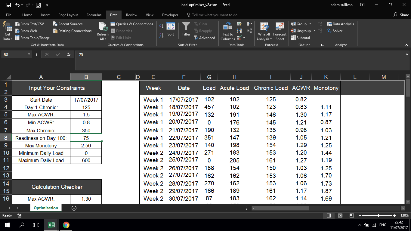
To start with, we need to set up a series of data to get our daily, acute and chronic load, as well as our a:c ratios and monotony values. This is all just manual input. I have previously shown, as well as provided downloads, on how to calculate acute to chronic loads and ratios using EWMA, so I won’t go through it again here. I will purely focus on using Solver and setting up shortcuts to use solver in this post.
You just need to put in the data and equations for calculating the previously mentioned headings, to get your data set. This will be the data that the constraints will be calculated from, and that Solver will manipulate to comply with these constraints.
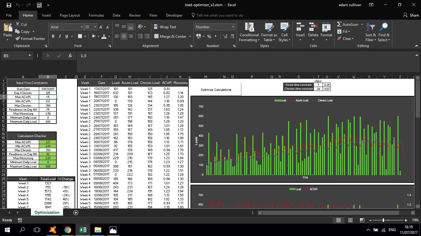
To set up the constraints, we need to set up a small series of cells, with values for total load, minimum & maximum ACWR, max training monotony, max chronic load, readiness on day 100 as well as minimum and maximum daily loads.
I have given this data set the heading of calculation checker, as I will later format this data to highlight when Solver has met our desired constraints.
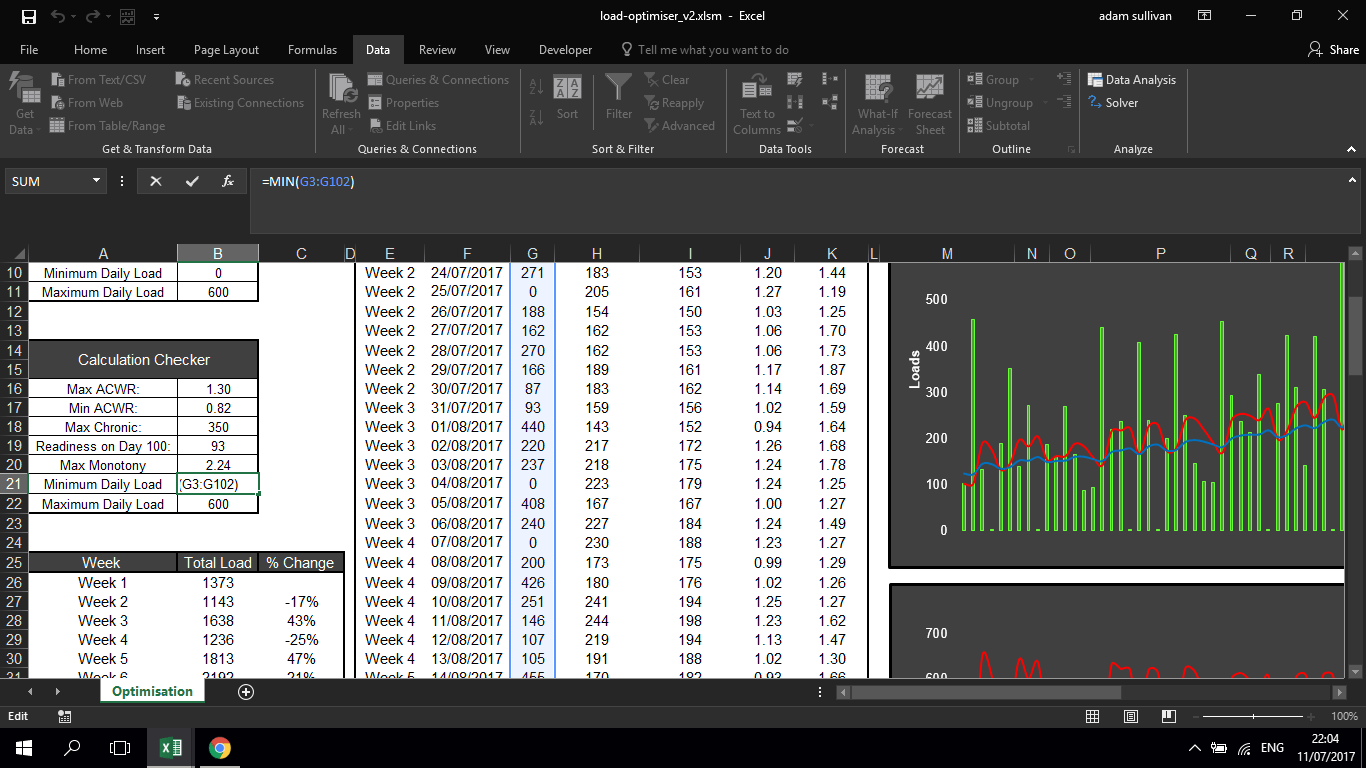
These cells will have formulas that calculate the total, maximum or minimum of each variable they are assigned to. So, for total load, we just sum up the entire load column: =SUM(G3:G102)

For maximum and minimum daily loads, the equations are as follows, respectively: =MAX(G4:G106) =MIN(G3:G102)
This style of max and min equation will continue for max and min ACWR, max monotony and chronic load.
Readiness on the last day will be the chronic load minus the acute load for that day:
= I102-H102

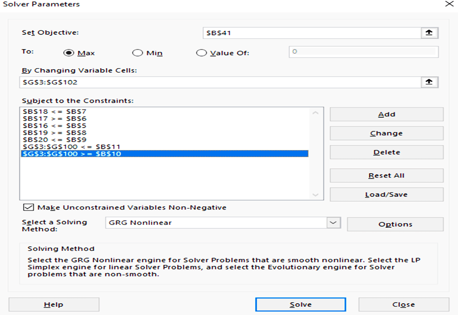
Next, we need to open Solver. You will enter your constraints in the solver parameters menu. We need to fill in the set objective box, the by changing variable cells box and the subject to the constraints box.
The objective in this project, is to maximise training load while keeping everything constrained by acute to chronic ratios and monotony. Every constraint will have its objective set to cell B41 (the total load cell).
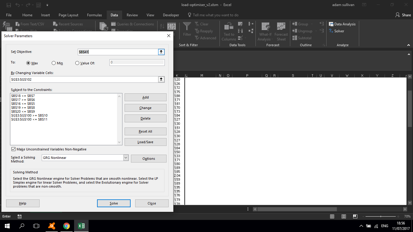
The by changing variable cells box, refers to the cells that will drive the calculations and constraints. Naturally, this will be the cell that contains the daily training load, since this drives the acute to chronic calculations etc. This range will be the cell range G3:G102.
You can see in the picture below the second table to the left named “calculation checker”. This group of cells has our calculations for each variable (max, sum, min etc.).
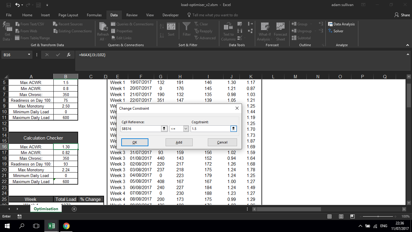
Traditionally when using Solver, you would click each of these cells and then add in a constraint. For example, my max ACWR would ideally be 1.5, so I would make my cell reference B16, which has the equation =Max(J3:J102). Then I would enter in a value that I want B16 to be less than or equal to, so I put in 1.5.
This is where Solver works it’s magic, I have already calculated what the maximum acute to chronic ratio value is in the data set in cell B16. Your data set could end up showing a maximum value of 1.7 when you calculate your max value.
However, now solver will realise that you’ve put a constraint on the data which won’t allow a value of 1.7 to be present in cell B16. So, it will manipulate the variable cells (daily training loads) to make sure your criteria of 1.5 is met.
This is how Solver works in a nutshell, you present the data first, then you manipulate it.
This process continues for each constraint:
ACWR 0.80-1.50
Max training monotony: 2.5
Max chronic load: 350
Readiness on day 100: >=50 (i.e., less fatigue than fitness by the very end of pre-season, in preparation for the first match).
Daily loads: 0-600 AU
A starting chronic load on day 1 of 125 AU.
This is how the solver parameters box looks when filled with different constraints.
You will notice that none of the cells refer to a value, but to another cell. What I have put together is a way to bypass solver, create your own constraints table, and just change the cell references to your liking, as opposed to going into solver each time to do so.
This is manually put in, but what I’ll do is instead of setting the constraint for cell B16 to have a maximum a:c ratio of 1.5, I’ll simply tell excel to ensure cell B16 is less than or equal to the value in cell B5, which I can change at will.
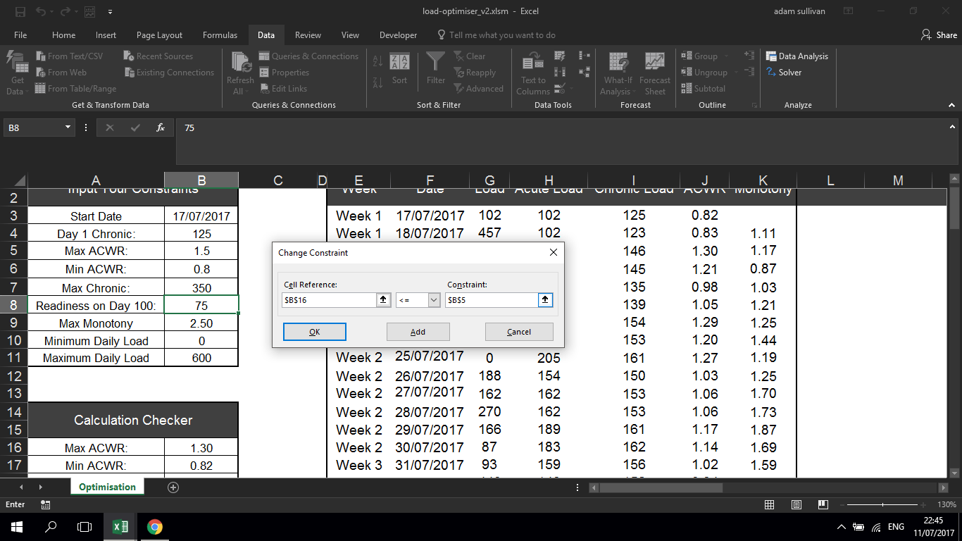
So, when I change the value in cell B5, excel just needs to ensure B16 is less than the value I put in B5. The example below shows that the constraint has been followed and B16 has calculated the maximum value in the data set to be 1.3.

I’ll continue this process by matching every cell reference to the cell where I’ll be able to manually input data. So, I’ll ensure that the cell reference in B17 (Min ACWR) is greater than or equal to cell B6. Use the picture above and below this text to see how I have matched the constraints to each cell.
Now that I have all my constraints built into solver, I can manipulate the constraints box as I please. However, I still need to click into solver and click solve each time I want to change the data.
I’ve avoided this by adding a simple button and some VBA code so I can just click once to get solver to run in the background.
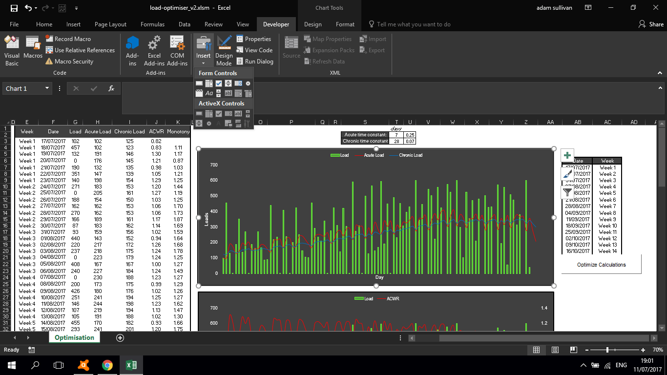
On the Developer ribbon, Control block, click on the Insert option to display Control options. Click the ActiveX Control Command Button icon. Drag a box on the worksheet to create a Command Button.
While the button is still selected, click the Properties icon on the Controls block. In this dialog box, set the (Name)=RunSolver. This will be the name of the Visual Basic subroutine that you will create and that the button will call when clicked.
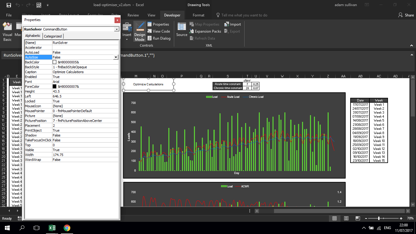
I’ve set the Caption= Optimize Calculations. This is the label that will be displayed on the button. Set TakeFocusOnClick=False.
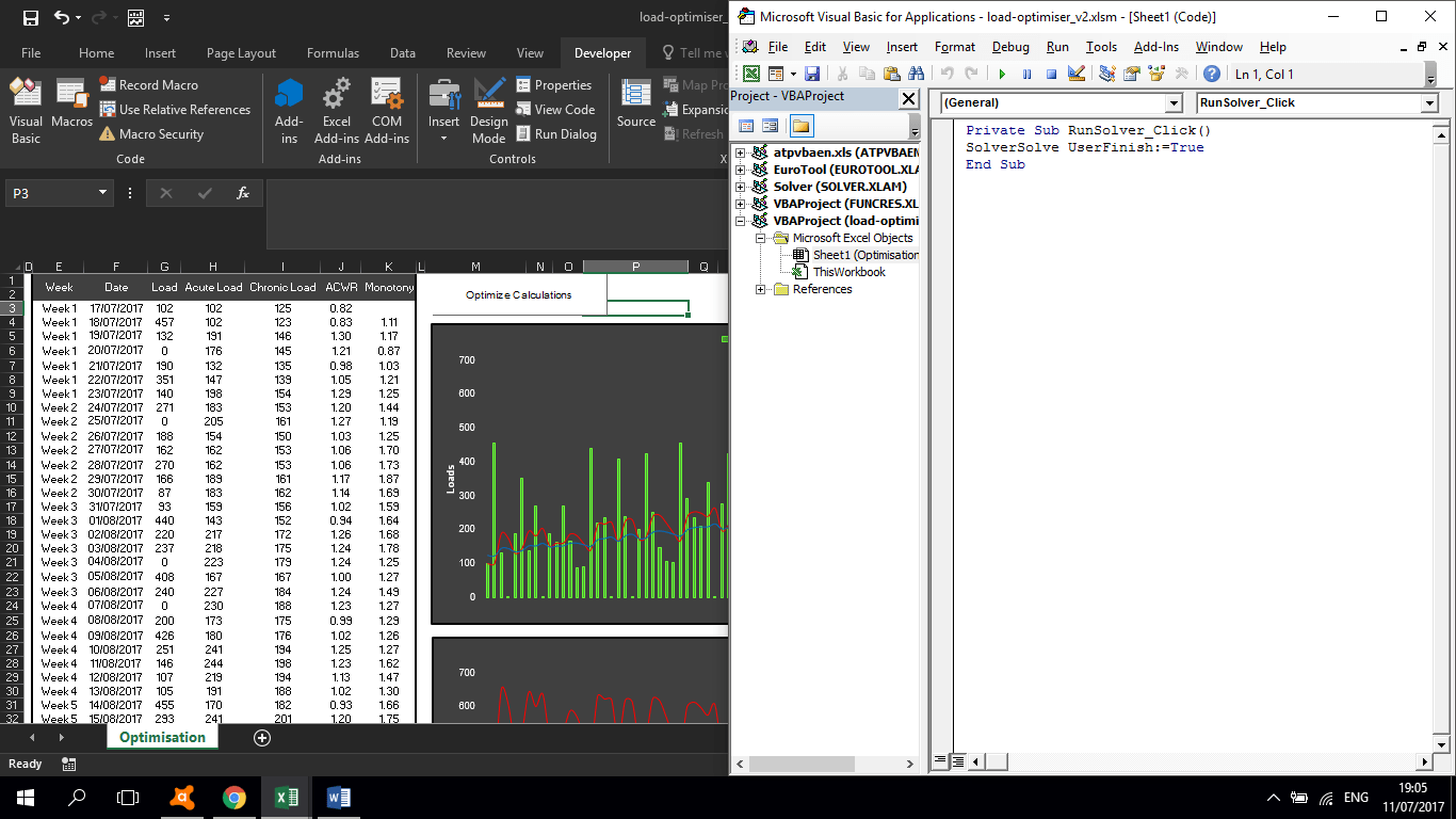
While you are still in design mode with the button selected, double click on the Command Button. This will open the Visual Basic Editor. You will be in an empty Private Subroutine called RunSolver_Click(). Enter the following command into the subroutine:
SolverSolve UserFinish:=True
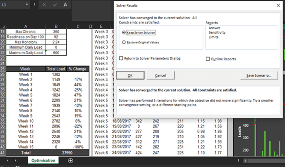
When you click solve in the solver parameters box, and everything goes smoothly, this message will pop up:
While you are still in the Visual Basic Editor, select the TOOLS menu and the REFERENCES option. Make sure that the solver.xls option is checked on the displayed dialog box and press OK.
Now, click on the Optimize Calculations button. The worksheet should quickly optimize without a solver dialog box showing up.
This new macro tells Solver to solve the problem without displaying the usual Solver Results dialog box. What this means is that solver will still run the optimisation, but it won’t tell you if it meets or fails to meet all constraints.
I’ve found that if the constraints aren’t met, it is usually only by a small margin.
The calculation checker box becomes a good reference here to see if your constraints have been met. I’ve added in some conditional formatting to highlight when the results have met the constraints I put in.
It is worth noting that, if you want to add in or change the constraints, you will still need to go back into solver to set up a new constraint. You can use the same format I have, to match the constraint value to the value you put in another cell.
You must also be wary of adding in too many constraints, as this will make it impossible for solver to find a solution. I have tried to have a constraint of keeping weekly load changes to below 10%, which failed miserably.
But, I manually created a % weekly load change table, because I can still manipulate the daily training loads once they have been optimised.
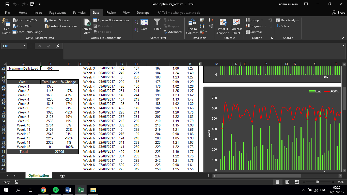
As you can see below, you can change the loads that solver has provided, if you wish to bring the % weekly load change down or up (or add in an extra rest day for example).
I’ve added in some conditional formatting to highlight when my manipulations violate my a:c ratio threshold.
This is the value of this tool, it’s not going to spit out a perfect loading pattern to follow to the letter, but it gives a nice template that you can modify to suit your training/match schedule.
You can also manipulate how the a:c ratios are calculated, by manipulating the acute and chronic time constant.
As mentioned before, some practical applications of such a tool could be:
- Changing the training loads to gps total distance or another metric of your choice. That might allow coaches to see what may occur when you increase you ACWR max to 1.7, for example. You may end up seeing that you cover an extra 10 km in total distance across the pre-season period at this ratio.
- Planning a safe return to play protocol, perhaps by using more strict ratios and max training loads.
- Developing a training plan that maximises performance/fitness whilst keeping within specific acute to chronic ratios or other variables that can reduce risk of injury.
Add in some nice charts to show your data and your good to go!
Hopefully this is of use and maybe inspires some improvements that could be made on this sheet too, if you have any suggestions or ways to use it be sure to get in touch!
PLEASE NOTE – I’ve had some issue uploading a macro enabled file to this website. I’ve managed to find a work around. When you click on the link for this file that says “click to download”, on the free downloads page, you will be taken to a dropbox page with the file on display. If you click on the download button in the right hand corner and select direct download, your download will start and you’ll have the workbook open in a matter of seconds!
Click here to be taken to the free downloads page to get access to this spreadsheet
Again a big thanks to Sean Williams @statman_sean, for giving me the chance to work on this and share it with you.
Enjoy!
