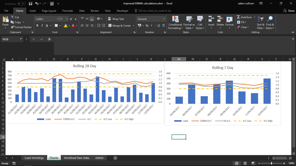
In my previous worksheets and demonstrations, EWMA calculations have required you to build an average or copy the first day’s workload to build up some data for the EWMA formula to work from. In previous downloads I have put out, when adding in a new athlete, you would have to change the formulas manually to ensure the first time an athlete’s name appeared, their load in the EWMA column would match their raw score. As seen below, the second time an athlete appears, the formula for EWMA could kick in.

I struggled for a while to make this process as automated as possible. I built some formulas that made sure every athlete had a corresponding daily date beside their name, to ensure a 0 value was put in for them, if no raw workload data was available. Thus, ensuring rest days were accounted for in the calculations.
I tried a simple formula to ensure that the first time an athlete displayed a value above zero, the formula would take this as the first days load to build the EWMA equation from, as if you took the first date entered for the entire team as the first load, it could be a zero (because the athlete may have missed the session) and that would skew the formula’s output going forward for that athlete.
So, I created a formula that allows you the option of giving every athlete an individual start date, this will be the first date a workload will be entered for this athlete, as not everyone may start on the same day.
To do this I first had to modify a previous formula that added a day onto each previous date for an athlete, which required a helper column to do so. The helper column works as follows:
=N(COUNTIF($E$4:E4,E4))
This formula continues down each cell. You can hide this column until it needs to be dragged down further.
This helper column basically displays the amount of times an athletes name has occurred, this allows the date formulas to pull the start date for each athlete when the helper column indicates it is the first occurrence of an athlete, this is indicated by a 1.
The date column then analyses whether it is the first occurrence for the athlete, which means it should display the start date, otherwise it should use the index and match function to match the athletes name to the last previous occurrence of their name (which uses the countif helper column). It then matches the date of this previous occurrence for this athlete, and adds a 1 onto this date, so you get a day by day progression for each individual athlete based on their start date.
{=IF(C16=1,VLOOKUP([@Player], Admin!$F$4:$G$104, 2),INDEX($D$4:D15,MATCH([@Count]-1&[@Player], [Count]&athlete, 0))+1)}
This is an array formula, so it needs to be activated by hitting ctrl+shift+enter.
Once the dates are in place and progressing for each athlete as planned. The EWMA formula is required for each timepoint, in my case 28 and 7 days.
This formula uses an IF and VLOOKUP function to ensure that the first date entered in the workings tab, matches the first date assigned to that athlete. If these dates match, then the EWMA box will just display that raw load figure. Otherwise, it will run the EWMA calculations.
This means that no matter what date the athlete starts, the first load will always be the raw workload score, and the following workloads will be dumped into the EWMA equation. This means that there is no need ot manually manipulate the data when new athletes are added in or if they start on different dates than the rest of the squad. Making calculations seamless.
The formula is as follows for EWMA 28day calculations:
=IF([@Date]=(VLOOKUP([@Player], Admin!$F$4:$G$13, 2, FALSE )),[@Load], SUMIFS(‘Load Workings’!$F$4:$F$7003,’Load Workings’!$E$4:$E$7003,’Load Workings’!$E4,’Load Workings’!$D$4:$D$7003,”<=”&’Load Workings’!$D4,’Load Workings’!$D$4:$D$7003,”>”&’Load Workings’!$D4-1)*$S$8+((1-$S$8))*SUMIFS(ewma28, athlete, E4, date, D4-1))
Just make sure you adjust the admin part of the equation to take in more athletes – Admin!$F$4:$G$13, won’t cover 20 athletes, so expand the range!
I have previously used an array formula for EWMA calculations too, but this improved formula doesn’t require an array, which makes things a lot faster in an excel file!
See the download here and try it out!
